QDO charge densities

libMBD can evaluate the charge density of the quantum Drude oscillators (QDOs) that underlie the MBD model, both without the dipole coupling (nonint_density()) and with it (int_density()). Both take a set of points and the QDO parameters and return the density at those points, so plotting is just a matter of choosing a grid. The underlying derivation is given in J. Hermann, Towards unified density-functional model of van der Waals interactions, PhD thesis, Humboldt-Universität zu Berlin, 2018, doi:10.18452/18706, Ch. 4, §4.3.1 (charge density) and §4.3.2 (first-order perturbation correction).

The QDO parameters follow from the vdW parameters via \(\omega_A=\tfrac43 C_{6,A}/\alpha_{0,A}^2\) and \(\alpha_{0,A}=q_A^2/(m_A\omega_A^2)\). The MBD convention sets \(m_A=1\), which gives \(q_A=\omega_A\sqrt{\alpha_{0,A}}\). The interacting density additionally needs the coupled MBD normal modes, obtained from a geometry constructed with get_spectrum=True. Both densities integrate to \(\sum_A q_A\).

The following minimal example evaluates both densities of an argon dimer along the bond axis and plots the non-interacting density together with the change induced by the coupling, using Matplotlib:

import numpy as np
import matplotlib.pyplot as plt

from pymbd import ang, from_volumes
from pymbd.fortran import MBDGeom

# argon dimer along z, 4 Å apart
coords = np.array([[0.0, 0.0, 0.0], [0.0, 0.0, 4 * ang]])
alpha_0, C6, R_vdw = from_volumes(['Ar', 'Ar'], [1.0, 1.0])

# QDO parameters (mass = 1 convention)
omega = 4 / 3 * C6 / alpha_0**2
m = np.ones_like(alpha_0)
q = omega * np.sqrt(alpha_0 * m)

# line of points along the bond axis
z = np.linspace(-3, 7, 500) * ang
pts = np.stack([np.zeros_like(z), np.zeros_like(z), z], axis=1)

# non-interacting density
rho_0 = MBDGeom(coords).nonint_density(pts, q, m, omega)

# interacting density, needs the coupled MBD modes
geom = MBDGeom(coords, get_spectrum=True)
_, eigs, modes = geom.mbd_energy(alpha_0, C6, R_vdw, beta=0.83)
rho = geom.int_density(pts, q, m, np.sqrt(eigs), modes)

# the coupling effect is tiny, so plot it against the non-interacting
# density on a separate axis
fig, ax = plt.subplots()
l1, = ax.plot(z / ang, rho_0, color='C0', label='non-interacting')
ax.set_xlabel(r'$z$ (Å)')
ax.set_ylabel(r'$n_0(z)$ (a.u.)', color='C0')
ax.tick_params(axis='y', labelcolor='C0')

ax2 = ax.twinx()
l2, = ax2.plot(z / ang, rho - rho_0, color='C1',
               label='interacting − non-interacting')
ax2.set_ylabel(r'$n(z) - n_0(z)$ (a.u.)', color='C1')
ax2.tick_params(axis='y', labelcolor='C1')

ax.legend(handles=[l1, l2], loc='lower center',
          bbox_to_anchor=(0.5, 1.0), ncol=2, frameon=False)
fig.tight_layout()
plt.show()

which produces:

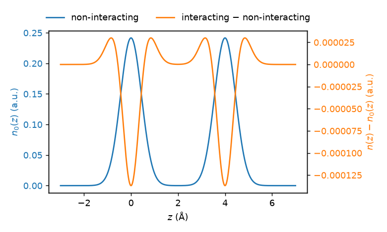
Non-interacting QDO charge density of an argon dimer (left axis) and the change induced by the dipole coupling (right axis), along the bond axis.

For a weakly bound system such as the argon dimer the coupling barely perturbs the density — note the four-orders-of-magnitude difference between the two axes. The coupling depletes density at the oscillator centers and shifts it into the bond region; the effect grows for more polarizable, strongly coupled systems.